Welcome to our project presentation of Neural Networks for object recognition, presenting a fully developed model trained by the CIFAR-10 image dataset by Keras.

 First a bit of background on Artificial Intelligence and object recognition.

 AI is the science of simulating human intelligence in machines by programming them to 'think', 'learn' and 'perform’ tasks in a way that humans would. AI is a discipline that uses different technologies, such as machine learning, computer vision and natural language processing. AI-enabled systems can process big data, and spot underlying patterns for important decision making. So we can think of AI as "the science and engineering of making intelligent systems" (IBM, N.D.).

 With AI being ubiquitous, the effects of AI on global economies are worth mentioning. While AI will replace jobs in areas such as agriculture technologies, e-commerce, and digital trade these job displacements are offset by job growth in other areas like climate change and environmental management solutions, big data, and cyber security. According to the World Economic Forum in this year’s report, this offsetting results in a net positive over the next five years (World Economic Forum, 2023).

 So varying fields of AI present great interest, with computer vision and object detection being the main focus of many industries.

 From retail, with self-checkout stores, to the automobile industry with self-driving cars, the division of AI which relates to allowing machines to 'see', is booming.

 Here we see an example of how a machine might separate different objects for detection, this is where our focus will be today.

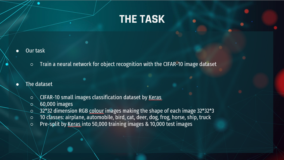
 Because we have been tasked to harness the power of discussed AI to train a neural network for object recognition with the CIFAR-10 small images classification dataset by Keras.

 This dataset consists of a total of 60,000 32*32 RGB colour images, evenly split over the 10 classes at 6,000 images each. The dataset has been pre-split by Keras into 50,000 training images, and 10,000 test images. We have been challenged to create a model that accurately classifies the test images into their respective categories.

 As seen here in the top right corner, we created a validation set from the training set by splitting the training set of 50,000 images with the `train_test_split()` function from the `sklearn.model_selection` module into an 80/20 train/test split. We set ` random_state` to 0 to ensure that the splits are equal each time we run the code.

 The reason we used a validation set is to avoid overfitting as a consequence of re-using the test dataset whilst tuning the models architecture and hyperparameters, for example by exploring the optimal number of hidden layers or different activation layers. The validation set also allowed us to implement an “early stop” function, this helped us determine when a model’s performance started to decline - indicating overfitting. This saves time and computational power by not running any unnecessary epochs. We then perform a final test on unseen data. Like Russel & Norvig said, we use “A test set to do a final unbiased evaluation of the best model”.

 Cross-Entropy is the most commonly used choice for classification problems as it has been found to work very well on these types of models. Since we are dealing with categorical data, we have applied the Categorical Cross-Entropy loss function (Brownie, 2019; androidkt, 2023) - the formula is displayed here in the middle of the screen and measures the dissimilarity between the true distribution and the estimated distribution, a measure to establish confidence in the classification model.

 Furthermore the data is preprocessed to normalise the pixel values to a value between 0 and 1 by dividing by the maximum RGB value of 255. This will aid the neural network in processing the input images.

 The output of the neural network will be a probability distribution over the classes, and to match this format, the labels are transformed to one-hot encoding. This allows for a more direct comparison between the neural network’s output and the true labels.

 In the final structure of our ANN there are 2 hidden layers each consisting of 1,000 neurons. Both of these layers use ELU as the activation function, `he_uniform` as the kernel initialiser, and `truncated_normal` as the bias initialiser.

 We explored multiple activation functions for the hidden layers such as Sigmoid, tanh, RELU, and Softmax, but found that ELU showed the best performance in our model. We did start out with Relu, but then we came across ELU which according to the literature has the potential for higher accuracy than RELU, albeit more computationally expensive (Himanshu, S., 2019; DJ, 2020)

 By looping through parameter permutations, which will be discussed on the next slide, we ascertained which activation function and kernels could provide optimal model performance.

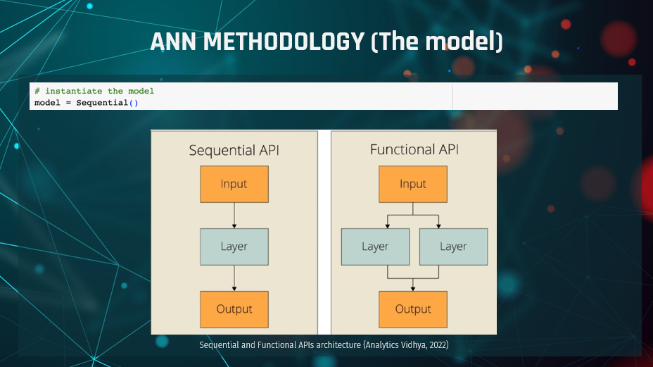
 As shown in the “ANN Design” section, the first decision in our design was which model to use. Generally speaking, Keras provides two different APIs related to modelling, the “Sequential” API and the “Functional” API. The “Functional” model is primarily used in complex problems with multiple input sources and output targets, with more than one input sensor and output sensor needed, when layers need to be shared or when “non-linear topology” is involved.

 In contradiction, the “Sequential” model is used in simpler problems with one input and output tensor, one input source and output target, and uses simple layer stacking while it is considered appropriate for more problems (Keras, 2020).

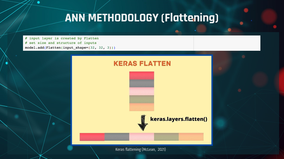
 Following the selection of the model, we started building the required layers. The first layer built resulted more from code requirements than from analysis. While the images were loaded by code, the output's shape differed from the required 1-dimensional input required for the input tensor/layer. By exploring the “input_shape variable”, we can understand that the initial input had three dimensions, with 32 elements in the first two dimensions and three in the third, which, in our case, represents images with RGB values of 0-1 float.

 After flattening the inputs, the output is of one dimension with 3,072 elements (having unrolled the three dimensions of 32x32x3), which is acceptable input for the layers-to-come.

 Providing the input as is through a multidimensional input/tensor may be technically possible. However, for such a volume of images, this process would have needed to be more convenient and not as computationally expensive (EDUCBA, 2023).

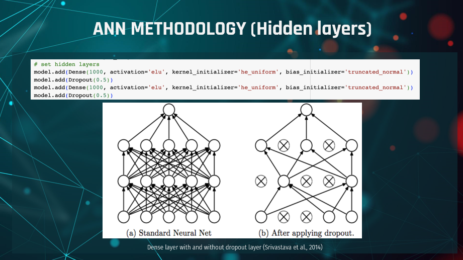
 As the input layer/tensor is now in the required shape and format, we then had to investigate the required hidden layers. By specifying two of the hidden layers as Dense (1st and 3rd line of code), we instructed the code that every neuron of the layer should receive input from all the neurons of the previous layer. The Dense layer is also commonly used for image classification, thus serving our purpose (Dumane, 2020).

 In between the Dense layers, we have also included a Dropout layer. A dropout layer is not adding another layer in the process per se (as seen in the second image) but affects other hidden or visible layers, such as the two Dense/hidden layers in our case. Dropout layers prevent overfitting and provide the capability of "combining exponentially many different neural network architectures efficiently" (Srivastava et al., 2014). In our case, the dropout rate is set to 0.5 float, effectively dropping 1 out of 2 (or 50%) of the input units.

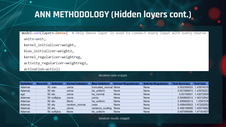
 From all the layers already discussed, the most interest is concentrated around the two Dense layers. This is because of the number of arguments available, the research performed, and how we selected the used activation and initializers.

 According to the available documentation, Dense layers can accept arguments such as the units (neurons), the activation function, kernel and bias initializers, regularizers and constraints, and activity regularizers. To find the best model for our data, we worked with the test dataset with early stopping (as explained earlier) on the number of epochs and a set number of neurons, by iterating through the different options. Our code iteration initially used four different kernel and activity/output regularizers. Considering that the regularizers apply a penalty, the outcome signified that no penalty was needed (Keras, 2020).

 At the same time, we iterated through 12 different initializers (applying random weighting through different methods) in the kernel and the bias. Several initializers were proven to perform the best, with marginal differences, such as the zeros kernel initializer with truncated normal, he uniform or he normal bias initializer.

 Activations are also an essential part of the hidden layers as they are essentially the data transformation functions of the input data to output data (ProjectPro, 2022). Our iteration tested nine different activation functions with selu (Scaled Exponential Linear Unit), elu (Exponential Linear Unit) and softmax (which applies probability distribution) performing marginally better.

 The argument exploration was one of the most critical parts of the project, as it allowed us to narrow down the available argument values to the most interesting and better-performing ones.

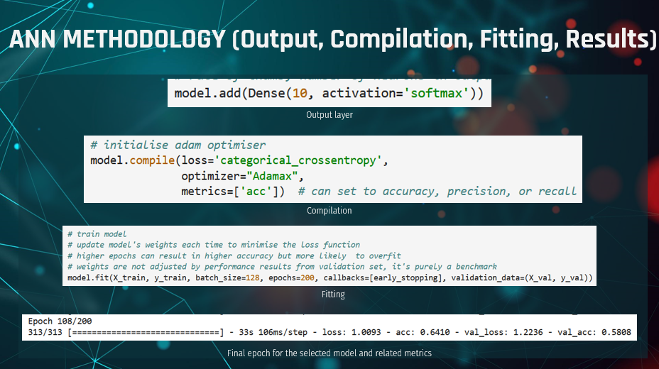
 As far as the model optimisation goes, after defining the input and hidden layers, we also had to define the output layer. The output layer followed the previous convention of using a Dense layer. The number of neurons was set to 10 to match the number of features in the classification problem. The output layer applies the softmax activation, as is the common standard, since this puts predictions in an interpretable probability format.

 After defining the output layer, we had to define the model compilation. The compilation instructions check for errors in the previously defined code and define the loss function, the activator and the metrics. The loss function used has already been explained in a previous slide, while for the optimiser, we followed the same approach of looping through different optimisers. Even though the Adam optimiser is the standard used, we discovered that Adamax, a variant of the Adam optimiser, performed better for our problem.

 Finally, on the accuracy argument, the accuracy was set by using the argument "acc". This allows the Keras library to handle the accuracy metrics based on the given loss function.

 Given that the used loss function was set to sparse categorical accuracy, the accuracy function used corresponds to the sparse categorical accuracy, which calculates how often predictions match integer labels (Keras, N.D.; Keras, 2019).

 On the model fitting part of the code, which tests how well the model performs in generalized data, based on the provided training, apart from the epochs used (for which we used early stopping), we also found the optimal batch size to be 128, to train the model on part of the data, then performing a gradient update and continuing with the next set/batch of data (Pramoditha, 2022).

  Even though iterations through the different arguments were performed, to find the best performing ones, the iterations limited the available options of the best parameter values. The iterations did not provide the final architecture, which is a product of manual trials on different numbers of layers used and different argument parameters based on the iteration results combined with discipline-specific knowledge and research. This resulted in an accuracy of 0.6410 and loss of 1.0093 in the training data, while in the validation data the model performed with an accuracy of 0.5808 and loss of 1.2236.

 The loss, representing the summarization of the errors, and in our model has a high value, even though the accuracy metric is above average, effectively representing a 0.58 (58%) accuracy, with significant errors, which may be explained by prediction outliers.

 During development of our ANN model it became clear that we were unlikely to be able to get it anywhere near to the 80-90% accuracy that were we looking for.

 Convolutional Neural Networks (CNNs) are excellent for image classification problems (Sultana et al, 2018). This is because the convolutional layers extract the features, as explained by Wang et al (2020), with each layer extracting ever more complex features.

 After checking with the tutor that it was OK to explore CNNs alongside ANNs, we started a parallel development to ensure that we were able to get a model to an acceptable accuracy figure for the project.

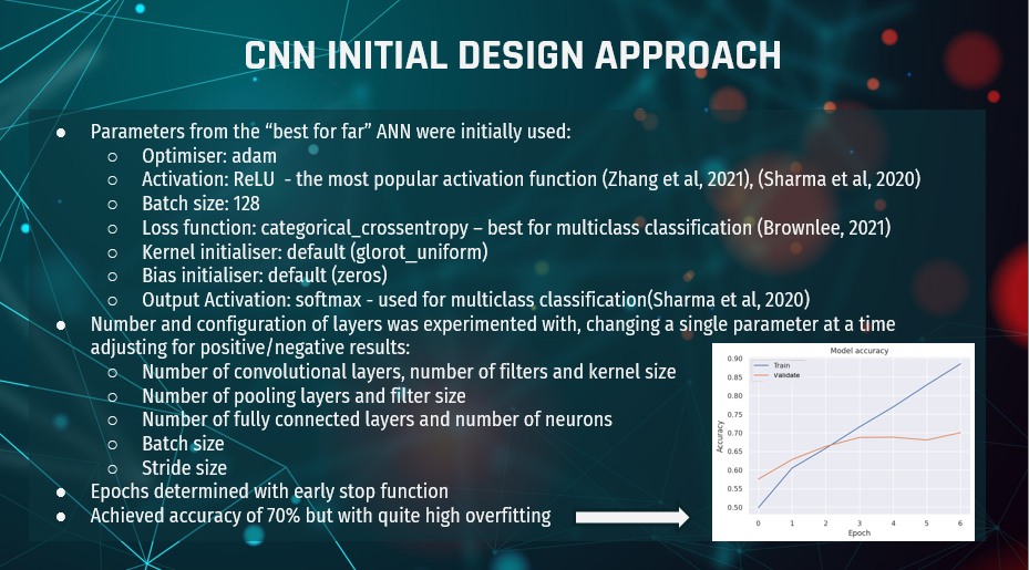
 Since we were already quite a long way through our ANN model development, we started the CNN with the “best so far” parameters from the ANN, which were:
 1. Adam for the optimiser, ReLU for the activation function, which is also the most popular activation function according to Zhang et al (2021) and Charma et al (2020), and batch size of 128.
 2. Categorical crossentropy loss function was used because it is considered best for multiclass classification problems according to Browlee (2021).
 3. Default kernel and bias initialisers of glorot_uniform and zeros respectively were used because we hadn’t selected optimal values from the ANN yet.
 4. Output activation softmax was used, as is standard for multiclass classification (Sharma et al 2020).

 With those parameters set we proceeded to experiment by changing a single parameter at a time, adjusting up or down depending the results. The parameters changed were:
 1. The number of convolutional layers and the number of filters and the kernel size within each layer.
 2. The number of pooling layers and the filter size of each pooling layer.
 3. The number of neurons and layers in the fully connected layers.
 4. The batch size.
 5. And the stride size.

 We used the early stop function again to determine the number of epochs.

 With this approach we got to around 70% validation accuracy as can be seen in the chart on the bottom right.

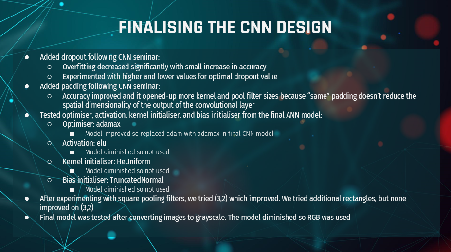
 Part-way through development the CNN seminar introduced dropouts and padding. We did a little more research and then incorporated both features into our model with immediate results. The dropout increased accuracy a little, but it significantly reduced overfitting, meaning we could push the models for longer to achieve better results. When we introduced “same” padding it also improved accuracy, but more significantly it opened-up more options for kernel and filter sizes because the convolutional layer was no longer reducing the spacial dimensionality of the output, which only started at 32x32 so didn’t take long to get to 1x1. We also discovered that the number of filters is generally a power of two (Dertal, 2017), with the number increasing with each layer due to the increasing complexity of the feature maps, so we started to adopt a 64, 128, 256 filters design.

 With results significantly improved, and the ANN model now finished, we applied any deltas from the ANN model to the CNN model to see if it could be improved even further. We found that changing the optimiser from adam to adamax improved the model, so we kept that change. The other parameters from the ANN model, being elo activation, HeUniform kernal initialiser and TruncatedNormal bias initialiser all diminished the model, so they were not used. We then tried a rectangular pooling filter of (3x2), having previously only tested square filters. Surprisingly, that improved the model, so we tested other rectangular filters, but they all diminished the model, so we kept the (3x2) filter.

 Finally, once we had the best model that we could get, we converted the images to greyscale to see if that made any improvement. The model diminished so we kept it at RGB.

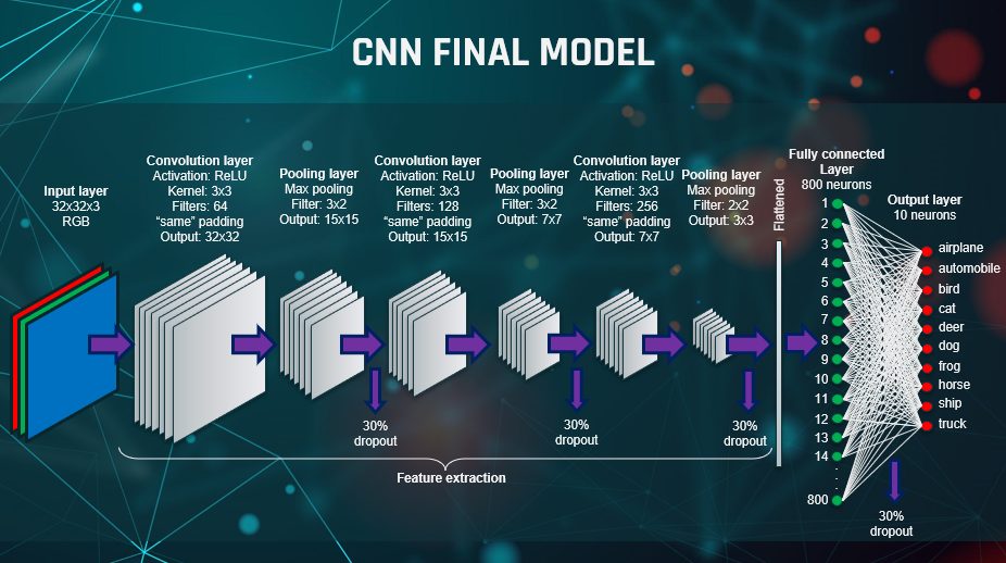
 This is a diagrammatic representation of our final model. It has:
 1. 32x32x3 RGB input
 2. 3 convolutional layers with (3x3) kernels and filters increasing from 64 through 128 to 256
 3. 3 pooling layers with filter size (3,2), (3,2), (2,2). The final filter size of (2,2) was to avoid the final output being 1x1.
 4. A fully connected single layer with 800 neurons
 5. A dropout of 30% after every pooling layer and after the fully connected layer
 6. A batch size of 128
 7. And ReLU activation

And not shown on the diagram, we had:  1. Adamax optimiser
 2. And Default kernel initialiser of glorot_uniform and bias initialiser of zeros

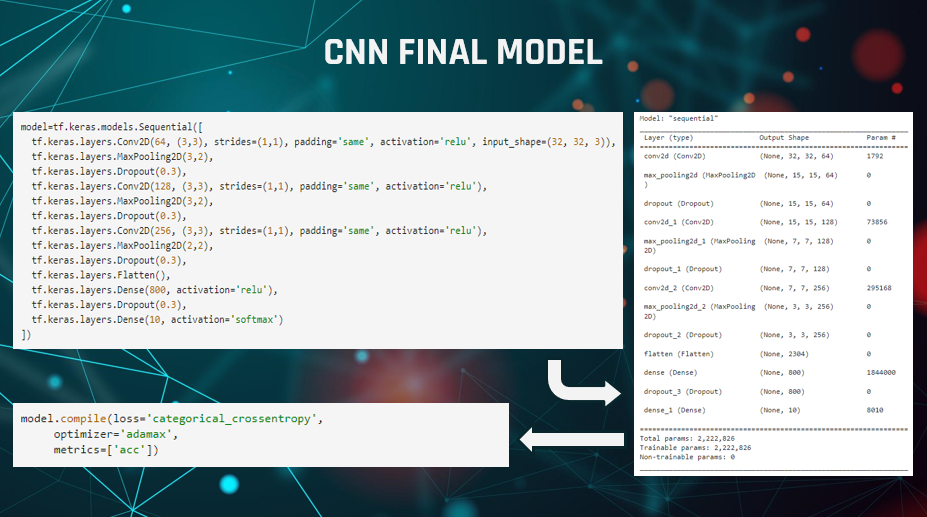
 Here are some code snippets of the final model to show how it was built. We can see on the right that the size going into the flatten layer is 3x3 as a result of the final pooling filter being 2x2 as explained before.

 So how did this model perform? Let’s find out on the next slide.

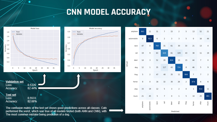
 We were really pleased to get an accuracy score of 82.44% against the validation set after 39 epochs, with a loss of 0.53. The loss and accuracy charts show a clear levelling-off but no marked downturn in performance.

 Most importantly, when the model was finally tested on the unseen test data set it achieved an accuracy score of 82.08%, so it was performing very consistently.

 The confusion matrix of the test results shows how well it matched each class individually. We can see that most classes scored very well, with ship being the best. The worst by some margin was cat, which was incorrectly matched with dog more than any other class.

 Overall, we felt it was a very good result.

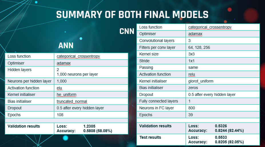
 Before we conclude, this is a summary of the final ANN and CNN models with their results. We can see, as already explained, the validation accuracy of ANN was 58% after 108 epochs and the validation accuracy of the CNN was 82% after 39 epochs, with test accuracy also of 82%

 As a team we were very happy with the final results of our ANN and CNN models. We got the accuracy as high as we were able to in the time given. Most importantly we all learned a lot about building neural networks.
The learning included:
 1. The functions of the hyperparameters and why tuning is key to model performance.
 2. That increasing neurons and layers can increase accuracy but can also lead to overfitting, and it increases computational demands.
 3. That dropout can be used to mitigate overfitting and increase accuracy.
 4. The structure of convolutional layers and pooling layers in CNNs and how to optimise them for image classification.
 5. That increasing epochs increases accuracy through backpropagation, but too many epochs leads to overfitting so the early stop function is useful to prevent that.
 6. And we learned that it’s actually quite easy to build machine learning models in Python using the Keras library.

 We felt that we worked very well as a team. We collaborated well, we were mature in how we divided the work, and we kept in regular contact.

 If there was one area that could’ve been improved, it was identification of a best practice set of parameters to start building the model from. We did search and found some pointers, such as ReLU being good for multiclass classification, but most literature suggested that trial and error is the best way to find an optimal model, which is what we did. We feel that with more research we might have been able to find a more specific set of starting guidelines though.